
Linux LVM explained
You can find bazillion sites explaining Linux LVM, however, I am preparing for my next article, about partition resize for the advanced user, and LVM deep understanding is required, so I have decided to explain some of the internals of LVM for the advanced user. This explains the how it is built more than the how to use it, so if you’re looking for the right commands – you are not likely to find them here. If you are looking for the theoretical understanding of how LVM is structured, what is PV, PE, LE and so on – this is probably an article you want to read.
In general, a block device – a disk, a partition, SSD, RamDisk, character device mapped as block (loop) or whatever – can be signed as a ‘physical device’ (PV) for the purpose of LVM. A physical device (from now on – PV) is a block device which can hold data and allow random access to it. For ease of definitions – a disk or its equivalent. If you can format and mount it – it can act as PV. The data this PV is required to hold is both the LVM metadata, and the PV ‘physical extents’ (PE). I will use the term PE.
The ‘Physical Extents’ are small partitions (logical definition, there is no ‘fdisk’ like tool to create them) the PV is being split to. It means that if we define a PE as a 32M chunk (this is a logical parameter when creating Volume Group. On that later), the PV will be split into many 32MB small chunks, each has its own number (sequential number, of course) in this PV. We will have PE #0, and PE#1 and so on. We, as humans, have (almost) no interaction with this numbering, but it is important we understand them.
All these ‘physical extents’ (PE) which reside on a ‘physical volume’ (PV) are mapped to a logical object called ‘logical volume’ (LV). A logical volume is the actual object we can use to place our data on. It behaves like any other block device or partition – we can format it, partition it (heavens knows why, but it can be done), mount it (when it has a file system), put our important data on – and so on. About how the mapping looks like – later in this article.
The connection between PE residing on a PV to the LV is kept in a logical object called “Volume Group” (VG). A “volume group” (VG) is a logical and theoretical object which merges the PE provided by multiple PVs into a logical group of objects with a mapping to the LV. This sounds complicated, I am sure, but we’ll get deeper into it soon.
As said – a VG is a logical object holding PVs (with their PEs) on one hand, and LVs (with their LEs, – about it later) on the other hand. It has no ‘real’ existence, except as a group of objects. A PV can be member of a single VG (but a single VG can have many PVs), and an LV can be a member of single VG (but again – a single VG can have many LVs). When we look at the metadata, later in this article, it should become more clear.
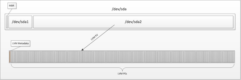
In order to understand how PEs are located on a disk, Let’s take a look at this nice drawing.
This drawing will show a (basic partitioning) disk, with Master Boot Record (MBR) and two partitions, of which the 2nd is used as LVM PV.
The PV has a small metadata signature, and many PEs.
We can ask the LVM mechanism nicely to export the metadata configuration. Since a volume group (VG) can hold multiple PVs (physical volumes, aka – block devices) the metadata will reside in the beginning of each disk (PV) for the sake of redundancy. This is important when we want to recover a failed LVM caused by human error or missing disk(s).
Moreover – because the LV has only logical mapping to the PEs residing on disks (can be more than one, and even more than three! ), the order of the PEs mapped to a single LV doesn’t have to be continuous, nor does it has to reside on a single disk. This is a flexible system, and we’ll get to that later.
I would like to show an exported (backed-up) VG metada for the sake of our observation. I will add comments inline for your viewing pleasure
# Generated by LVM2 version 2.02.98(2)-RHEL6 (2012-10-15): Thu Jun  5 00:00:00 2019

contents = "Text Format Volume Group"
version = 1

### This is the description of the command used to create this file ###
description = "vgcfgbackup -f /tmp/VG-export.txt VG00"

### Some information about the creation host and time ###
creation_host = "localhost.localdomain"	# Linux localhost.localdomain 2.6.32-358.el6.x86_64 #1 SMP Fri Feb 22 00:31:26 UTC 2013 x86_64
creation_time = 1594292258	# Thu Jun  5 00:00:00 2019

### Volume group information ###
VG00 {  ### Name of the Volume Group ###
	id = "8svbhm-euN1-d7Hr-PGIo-yHnH-kIIa-yxECBa"  ### Each object has unique ID to prevent confusion ###
	seqno = 8
	format = "lvm2" # informational
	status = ["RESIZEABLE", "READ", "WRITE"]
	flags = []
	extent_size = 65536		# 32 Megabytes ### The size of a single PE in Sectors. This is across all VG (all the member PVs), regardless of the PV size! ###
	max_lv = 0   ### Configurable limitations. None.
	max_pv = 0
	metadata_copies = 0

	physical_volumes { ### The list of the member PVs ###

		pv0 {  ### This is the first PV. They will have names like 'pv0' or 'pv1'. Nothing very artistic ###
			id = "FRDFDw-fMrG-ma1d-2rP5-bqck-cFsz-fr2OWf"   ### UUID. A unique identifier allowing for easy scan
			device = "/dev/sda2"	# Hint only ### This is only a hint. Device-mapper (LVM kernel engine) scans for LVM metadata on all disk partitions ###

			status = ["ALLOCATABLE"]  ### Can we allocate PEs from this PV? Why not? We can prevent it from allocating space. On that - some other time ###
			flags = []
			dev_size = 209590272	# 99.9404 Gigabytes ### The PV size in Sectors. This is very important. ###
			pe_start = 2048 # The offset of the first PE, #0, from the beginning of the PV, in Sectors ###
			pe_count = 3198	# 99.9375 Gigabytes # How many PEs do we have here? The size can be easily calculated by multiplying the amount of PEs (pe_count) with the size of each PE (extent_size)
		}
	}
I will go further into the LV topic shortly, but in the meanwhile – let’s see what we have here. This is the global definition of a Volume Group (VG) and its physical volume(s) (PV). The VG name is ‘VG00’ and it has a unique ID (which is why you do not want to map storage snapshost of an LVM to the same machine in parallel, without fully understanding what you are doing). We have the size of the PE – 32M in our case. As soon as the VG was created – it cannot be changed. A note – the PEs don’t have a header on-disk, meaning you cannot binary-dump a hard drive and look for the beginning or end of each PE. The PEs are defined as a mapping, and the driver can jump to the right location on the disk. It is fairly easy – calculate the position of the PE you aim at by multiplying the PE size with the sequential number of the PE, jump to this number relatively to the beginning of the partition, and you’re there.
Let’s look at the PV definition here – we have its UUID, which is extremely important, as it identified the PV for the VG. Since there is no order constraint on the devices (you can reverse the disk order for a multiple-PV system, and LVM will not get affected) – the only way LVM identifies the member PVs is by looking at their metadata copy, containing their UUID. If the metadata is damaged, missing or has an incorrect UUID, we get to data recovery! (or metadata recovery, which is easier, but still unpleasant).
Since the physical OS disk mapping doesn’t matter, because LVM makes use of PV UUID, the block device name is only a hint, for the human who might read this config backup file.
We have the status. A PV can be set to ‘not allocatable’ – let’s say we want to evict a PV from a VG – this can be done, however, in the meanwhile, we would not want anyone allocating data on this soon-to-be-removed PV – so we set it to ‘not allocatable’ to keep it empty.
It can have additional flags, used in cases of external lock management like in HA clusters.
Next, it shows the size of the device in sectors ; the PE beginning location (relative to the beginning of the PV), and the amount of PEs present in it.
Now, let’s look at how an LV is defined. Again – comments inline:
logical_volumes {

		lvroot {  ### The name of the LV ###
			id = "dmaQ5x-eTX0-JRsR-aMhG-Ldz5-SlR6-lAT6EB"  ### A unique identifier.  ###
			status = ["READ", "WRITE", "VISIBLE"] ### It is available R/W and visible. It can be none of these too ###
			flags = [] ### Special arguments. None defined ###
			creation_host = "localhost.localdomain"
			creation_time = 1594157738	# 2019-01-01 08:42:18 +0000
			segment_count = 1 ### An LV can be continuous or split in multiple ways. I will demonstrate that later ###

			segment1 { ### The first continuous are (and the only one, in our case ###
				start_extent = 0 ### Where does it start with the LOGICAL extent? On that later ###
				extent_count = 875	# 27.3438 Gigabytes ### The amount of LEs used by this segment, meaning - the segment size or length ###

				type = "striped" 	# linear  # There are multiple types. striped is the common one - a linear setup
				stripe_count = 1 ###

				stripes = [ ### Where does this segment reside *physically*? ###
					"pv0", 0 ### On 'pv0' we've seen before! And where does it start? On PE 0 (the first one) ###
				]
			}
		}

		lvswap { ### Another LV
			id = "E3Ei62-j0h6-cGu5-w9OB-l9tU-0Qf5-f09bvh"
			status = ["READ", "WRITE", "VISIBLE"]
			flags = []
			creation_host = "localhost.localdomain"
			creation_time = 1594157749	# 2019-01-01 08:42:29 +0000
			segment_count = 1

			segment1 {
				start_extent = 0  ### Tee LE of the LV. On LEs - later ###
				extent_count = 94	# 2.9375 Gigabytes

				type = "striped"
				stripe_count = 1	# linear

				stripes = [
					"pv0", 1813 ### Here we start at PE number 1813. More details below ###
				]
			}
		}
	}
Before I explain the LV settings, I need to explain what ‘Logical Extent’ is. A block device has to be presented to the operating system as a continuous device with random-access capabilities. So, logically, an LV has to be continuous. However – we do know that LVM allows us to modify, migrate and even resize an existing LV into split areas of a disk or disks (PVs). This is achieved by defining an LV as made out of a set of small chunks, ordered in a continuous manner. They are ordered in such a way, however, since they are logical, they can be mapped to any PEs we have, in a non-ordered mode. It means, practically, that this ‘chunk’, called “Logical Extent” (LE) is in the size of PE, and maps to one (or more, in cases of LVM RAID. Not included in this article). So an LV has a continuous array of LEs mapped to non-continuous list of PEs. This way, LVM can satisfy both the OS requirement for a block device, with the relevant properties, while maintaining flexibility with the actual disk positioning.
Here is another image to elaborate some more on the LE-to-PE mapping. This image was taken, with permission, from ‘thegeekdiary’ article explaining Linux LVM basics. If you want to know how to do stuff – you should check this article. I am just explaining how things look internally.
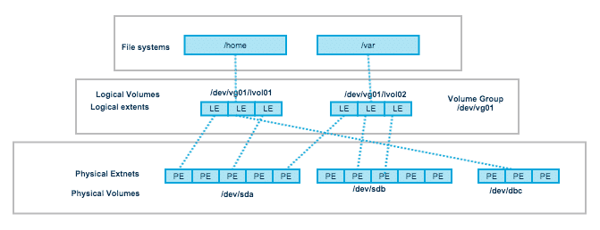
So – Back to our configuration. What do we have here? A Logical Volume (LV) is a logical unit with parameters, like name, UUID, status and so on. We can see that the LV called ‘lvroot’ has one ‘segment’ (called ‘segment1’). A segment is an uninterrupted list of continuous blocks, with a logical starting point and length (aka – uninterrupted list) with mapping of “extents” (in the configuration – meaning LE) to the starting point on the PV, defined as “PV”, PE_number. In this configuration, we can see that ‘lvroot’ block (LE) 0 begins at the PV ‘pv0’ block (PE) 0.
Here is aconfiguration dump of the same LV after I have migrated the first 10 PEs to another location in the disk (PV), using the command
pvmove –alloc anywhere /dev/sda2:0-9
lvroot {
                        id = "dmaQ5x-eTX0-JRsR-aMhG-Ldz5-SlR6-lAT6EB"
                        status = ["READ", "WRITE", "VISIBLE"]
                        flags = []
                        creation_host = "localhost.localdomain"
                        creation_time = 1594157738	# 2019-01-01 08:42:18 +0000
                        segment_count = 2 ### We now have two segments! ###

                        segment1 {  ### This is the beginning of the LV - mapped as LE 0-9 (the first 10, which I have migrated) ###
                                start_extent = 0
                                extent_count = 10       # 320 Megabytes

                                type = "striped"
                                stripe_count = 1        # linear

                                stripes = [
                                        "pv0", 1907 ### They are on pv0, but somewhere further back the disk, on PE 1907 and onwards! ###
                                ]
                        }
                        segment2 { # This is the next segment, of blocks 10 to the end ###
                                start_extent = 10
                                extent_count = 865      # 27.0312 Gigabytes

                                type = "striped"
                                stripe_count = 1        # linear

                                stripes = [
                                        "pv0", 10 ### It resides at the original location, which was PE 10 and onwards ###
                                ]
                        }
                }
The LV mapping has changed to match the change. The first 10 blocks (LEs) of lvroot are somewhere else on the disk on PV ‘pv0’ at location 1907, and the next segment of blocks remains in its original position – blocks 10 and onwards, except that because I’ve split the LV into two chunks, it has to have a new ‘segment’ definition.
This concludes my explanation of disk positioning and how it looks like, with LVM internals. We went through what PV is, what PE is, what LV and LE are, and how they are related to each other. Just to stress – a VG is a logical construct combining the PVs, PEs to the LEs and LVs.
If you find anything incorrect, not clear enough or want me to go further into any detail – drop me a note. I will be happy to hear from you.
One Comment